How Android Raw GNSS Works — and Why SIMT Builds Its Own Positioning Engine

Your phone already hears the satellites

Right now, as you read this, your phone is receiving radio signals from at least a dozen satellites orbiting about 20,000 kilometers above your head. These satellites belong to constellations operated by different countries and regions: GPS by the United States, Galileo by the European Union, GLONASS by Russia, BeiDou by China, QZSS by Japan, and NavIC by India. Each satellite broadcasts a precisely timed signal that travels at the speed of light. Your phone picks up that signal, measures how long it took to arrive, and uses the delay to estimate how far away the satellite is.

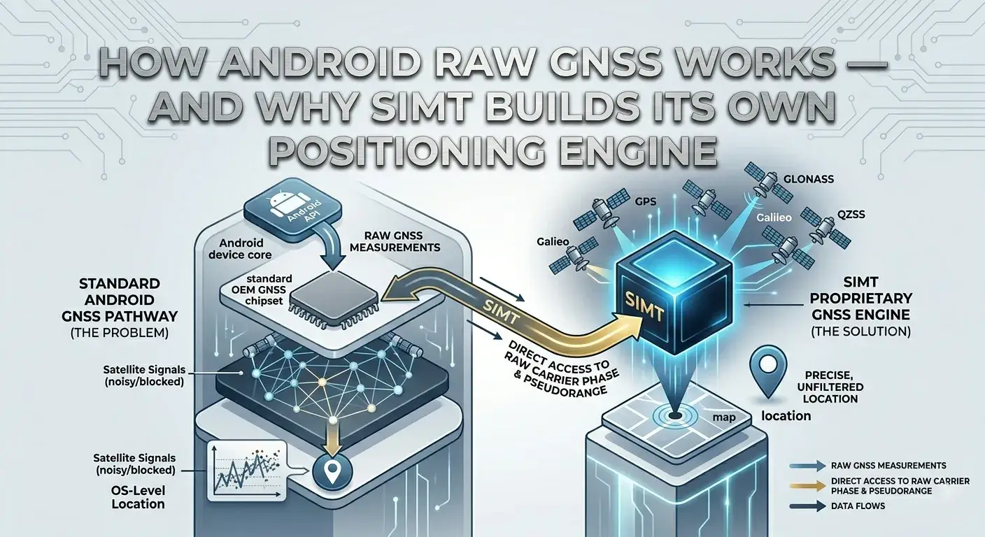
That distance estimate is called a pseudorange. It is called 'pseudo' because it is not a true geometric range — it includes errors from the satellite clock, the receiver clock, the atmosphere, and the signal path itself. With pseudoranges from at least four satellites, a device can solve for three spatial coordinates plus a clock offset. That is the fundamental idea behind satellite navigation. And since 2016, Android has made these raw timing measurements available to any app that asks for them.

The catch? Almost no app actually uses this data. The standard approach is to let Android's built-in GNSS chipset compute the position and hand the app a latitude, longitude, and accuracy estimate — a black box that works well enough for turn-by-turn navigation. But 'well enough' is a three-to-ten meter accuracy bubble that hides what the raw signals can actually tell you.

From timing to distance: how pseudoranges are born

When a satellite transmits its signal, it encodes the exact moment of transmission. Your phone records the exact moment of reception. The difference between those two timestamps, multiplied by the speed of light, gives you a distance. In Android terms, this involves reading nanosecond-precision fields from the GNSS clock and comparing them with each satellite's transmission time.

But the word 'exact' is doing heavy lifting. The satellite has an atomic clock accurate to a few nanoseconds, but your phone has a quartz oscillator that can drift by microseconds. A single microsecond of clock error translates to about 300 meters of range error, because light travels 300 meters in one microsecond. This is why the receiver clock offset must be estimated alongside your position in every solution epoch.

There are additional subtleties. Each constellation uses a different time reference. GPS runs on GPS Time, GLONASS uses UTC with leap-second adjustments and a different day cycle, Galileo uses Galileo System Time, BeiDou has its own epoch, and regional systems like QZSS and NavIC maintain their own time scales aligned to GPS Time but with independent offset terms. When you combine satellites from multiple constellations in a single solution, you need a separate clock bias term for each one — what engineers call inter-system bias, or ISB. A solver that ignores ISB will produce a position that looks reasonable but is quietly wrong by meters.

Knowing where the satellites are

A pseudorange tells you how far a satellite is. But to use that distance, you also need to know where the satellite was at the instant it transmitted the signal. Satellites are not stationary — they orbit the Earth at roughly 14,000 kilometers per hour. Their positions are described by orbital parameters called ephemeris data, which each satellite broadcasts as part of its navigation message.

For GPS, Galileo, BeiDou, QZSS, and NavIC, the ephemeris uses Keplerian orbital elements: a set of six parameters that describe the shape, tilt, and orientation of the orbit, plus correction terms for perturbations caused by Earth's uneven gravity, solar radiation pressure, and tidal forces. Given these parameters and a time, you can compute the satellite's position in Earth-centered coordinates using a well-defined set of equations from the system's interface control document.

GLONASS is different. It does not broadcast Keplerian elements. Instead, it sends the satellite's position, velocity, and acceleration at a reference time, and the receiver must propagate the orbit forward using numerical integration — specifically, a fourth-order Runge-Kutta method that accounts for Earth's gravitational harmonics and the gravitational pull of the Sun and Moon. This is more computationally expensive than the closed-form Keplerian approach, but it is necessary because GLONASS orbits are specified that way.

The atmosphere bends everything

The satellite signal does not travel through empty space all the way to your phone. It passes through two layers of atmosphere that slow it down and bend its path. Getting the distance right requires correcting for both layers.

The first layer is the ionosphere, a region roughly 60 to 1,000 kilometers above the surface where solar radiation strips electrons from gas molecules. These free electrons slow the GNSS signal by an amount that depends on the signal frequency and the density of electrons along the path. On a quiet day, the ionospheric delay can add 5 to 15 meters of apparent range. During a solar storm, it can exceed 100 meters.

For single-frequency receivers, the ionospheric delay must be estimated from a model. The most common is the Klobuchar model, which uses eight broadcast coefficients to approximate the delay as a half-cosine function of local time. It corrects roughly 50 to 60 percent of the true delay. The European Galileo system offers a more sophisticated model called NeQuick-G, which models the 3D electron density profile of the ionosphere and integrates it along the signal path. If you have dual-frequency observations — such as L1 and L5 — you can form an ionosphere-free combination that eliminates the first-order delay entirely, no model needed.

The second layer is the troposphere, the lowest 12 kilometers of atmosphere where weather happens. The troposphere delays the signal by about 2.3 meters at zenith and up to 25 meters at low elevation angles, because the signal travels through more atmosphere when the satellite is near the horizon. Unlike ionospheric delay, tropospheric delay does not depend on frequency, so dual-frequency techniques cannot remove it. Instead, it is modeled using surface pressure, temperature, and humidity. A common approach is the Saastamoinen model for zenith delay combined with the Niell mapping function, which scales the zenith delay to the actual satellite elevation.

More corrections than you expect

Atmospheric corrections are the largest error sources, but they are not the only ones. A precise positioning engine must also correct for several smaller but significant effects.

• Satellite clock error: each satellite carries atomic clocks that still drift slightly. The broadcast ephemeris includes polynomial coefficients to correct the clock offset, plus a relativistic term caused by the satellite's elliptical orbit.
• Earth rotation (Sagnac effect): while the signal travels from satellite to receiver, the Earth rotates underneath. For a transit time of about 70 milliseconds, this rotation shifts the receiver by roughly 30 meters relative to the satellite's transmitted coordinates. The correction requires knowing both the satellite and receiver positions.
• Relativistic effects (Shapiro delay): the signal passes through the gravitational potential well of Earth, which bends spacetime slightly and adds a small delay — typically a few centimeters.
• Differential code bias: if you combine signals on different frequencies, the hardware in the satellite and receiver introduces a small systematic offset between the code measurements. This bias must be accounted for when forming ionosphere-free combinations.

Each of these corrections is small individually. But in positioning, errors are cumulative and geometric. An uncorrected two-meter bias on one satellite propagates through the geometry matrix and can shift your computed position by five meters or more, depending on which direction the satellite is in.

SBAS: augmentation from geostationary orbit

Between the broadcast-only corrections described above and the precise internet-streamed products described later, there is a middle layer of augmentation that arrives directly from space: SBAS — the Satellite-Based Augmentation System.

SBAS is a set of regional systems that use geostationary satellites to broadcast real-time corrections and integrity information for GPS and other GNSS constellations. WAAS covers North America, EGNOS covers Europe, MSAS covers Japan, GAGAN covers India, and SDCM covers Russia. Each system operates a network of precisely surveyed ground stations that monitor the GPS satellites, compute corrections, and uplink them to GEO satellites for rebroadcast on the GPS L1 frequency. Any receiver that can track GPS L1 can receive SBAS corrections for free, with no internet connection required.

SBAS broadcasts several types of corrections in a 250-bit message format at one message per second. Fast corrections (message types 2 through 5 and 24) provide rapidly updated pseudorange corrections for each monitored GPS satellite, compensating for fast-changing clock errors. Long-term corrections (message type 25) provide slower-changing orbit and clock offsets that refine the satellite's broadcast ephemeris. Together, these corrections reduce the orbit and clock error budget from meters to well under a meter.

SBAS also broadcasts ionospheric corrections on a geographic grid (message types 18 and 26). Instead of the simple Klobuchar half-cosine model, SBAS provides measured vertical ionospheric delays at specific grid points covering the service area. A receiver computes where its signal pierces the ionosphere — the ionospheric pierce point — and interpolates the delay from the surrounding grid points. This grid-based approach is significantly more accurate than the Klobuchar model, especially during periods of elevated ionospheric activity. On a dual-band receiver, however, the SBAS ionospheric grid is not needed for ionospheric correction — the L1/L5 hardware combination already eliminates it without any external data. SBAS still contributes fast clock corrections, long-term orbit and clock offsets, and GEO satellite ranging, all of which remain useful regardless of how many frequencies the device tracks.

Beyond corrections, SBAS GEO satellites themselves can serve as additional ranging sources. Each GEO satellite broadcasts its own ephemeris (message type 9) as an ECEF position, velocity, and acceleration at a reference time. The receiver propagates the GEO position using a second-order Taylor expansion — simpler than the Keplerian model used for GPS, but appropriate for geostationary orbits that change slowly. Adding GEO ranging measurements to the solution improves satellite geometry, particularly at low latitudes where geostationary satellites are high in the sky.

Carrier phase: the precision signal most apps ignore

Everything described so far uses the code measurement — the pseudorange derived from the signal's timing code. Code measurements are relatively noisy, with a precision of about 0.5 to 3 meters under good conditions. But the satellite signal has another component that is far more precise: its carrier wave.

The carrier is a continuous sine wave at a known frequency — for GPS L1, it oscillates at 1,575.42 MHz, with a wavelength of about 19 centimeters. A receiver can track the phase of this wave with a precision of a few millimeters. That means carrier phase measurements are roughly a thousand times more precise than code measurements.

The problem is ambiguity. The receiver can measure the fractional phase within one wavelength very precisely, but it does not know how many whole wavelengths fit between the satellite and the receiver. This unknown integer is called the carrier phase ambiguity, and resolving it is one of the hardest problems in GNSS.

Even without resolving the integer ambiguity, carrier phase is useful. A technique called Hatch filtering uses the carrier phase to smooth the noisy code pseudorange over time. Each epoch, the filter blends the new code measurement with the change in carrier phase since the previous epoch. The result is a pseudorange that converges toward carrier-phase-level noise while staying anchored to the absolute scale of the code. This smoothing significantly improves position accuracy, even with consumer-grade phone antennas.

Solving for position: iterative weighted least squares

Once you have corrected pseudoranges from multiple satellites, you need to solve for your position. The relationship between your position and the pseudoranges is nonlinear — the geometric range between a point on Earth and a satellite in orbit involves square roots of coordinate differences. To handle this, the solver linearizes the problem around a guess of the receiver position and iterates.

At each iteration, the solver computes what the pseudoranges would be if the receiver were at the current estimated position, compares them with the actual measured pseudoranges, and solves for a correction to the position estimate. This is weighted least squares: each measurement gets a weight proportional to its expected quality. Measurements from high-elevation satellites with strong signal strength get more weight. Measurements from low-elevation satellites in poor signal conditions get less.

The weighting model matters more than most people realize. A satellite at 10 degrees elevation sees its signal travel through four times more troposphere than one at 90 degrees. Its signal is more likely to bounce off buildings. Treating all measurements equally would let one bad low-elevation observation drag the entire solution by meters. A good weighting model combines elevation geometry, signal-to-noise ratio, and bounded pseudorange uncertainty to keep the solver focused on the most trustworthy data.

The numerical method behind the solver also matters. The standard approach — forming normal equations and solving with Cholesky decomposition — works well when the observation geometry is strong. But when satellites are clustered in one part of the sky, the geometry becomes ill-conditioned, and the normal equations can amplify numerical errors. A QR decomposition approach is more numerically stable, handling the same geometries where Cholesky would fail or produce inflated position uncertainties.

Integrity and outlier rejection

A position solution is only useful if it is trustworthy. In the satellite navigation industry, trust is formalized through a concept called integrity — the ability to detect when something has gone wrong and warn the user.

The simplest integrity check is RAIM — Receiver Autonomous Integrity Monitoring. After the solver converges, each satellite's residual (the difference between the modeled and measured pseudorange) is examined. If a satellite's residual exceeds a threshold, that measurement is likely corrupted — perhaps by multipath, a clock jump, or a bad ephemeris — and should be excluded. The solver is rerun without the offending satellite, and the process repeats until all remaining residuals are below the threshold.

Beyond RAIM, the solver produces covariance information that yields dilution of precision (DOP) values. These describe how much the satellite geometry amplifies measurement errors. A low HDOP means the satellites are well-spread in azimuth and your horizontal position is well-determined. A high HDOP means the geometry is poor and you should treat the result with more caution. The final reported accuracy combines the post-fit residual statistics with the geometry to give a realistic uncertainty estimate.

Smoothing across time: the Kalman filter

Each epoch's weighted least squares solution is independent — it uses only the measurements available at that instant. But in practice, you know something about how a receiver moves: it does not teleport between epochs. A Kalman filter exploits this continuity by maintaining a model of position and velocity, and blending each new epoch's solution with the predicted position from the motion model.

The result is a position that is smoother and more robust than any single epoch could provide. Temporary measurement dropouts, brief multipath spikes, and natural noise are absorbed by the filter's memory of where you were and how you were moving. The filter also helps identify outlier epochs: if a new WLS solution disagrees wildly with the predicted position, the filter can flag it rather than blindly accepting it.

Pushing beyond broadcast: RTK, PPP, and integer ambiguity resolution

Everything described so far uses broadcast corrections — the parameters transmitted by the satellites themselves, plus any SBAS augmentation. Broadcast ephemeris limits orbit accuracy to about one meter, and broadcast clocks to about two meters. These are the dominant error sources once atmospheric corrections are applied. To break through this floor, you need external precise products — and there are two fundamentally different approaches.

The first approach is RTK — Real-Time Kinematic positioning. RTK uses a nearby base station at a precisely known location that observes the same satellites as your phone. The base station streams its raw observations to your receiver over the internet using the NTRIP protocol. Because the base and rover see the same satellites through nearly the same atmosphere, most errors cancel when you form differences between their measurements. With a base station within 30 to 50 kilometers, ionospheric, tropospheric, orbit, and clock errors largely vanish, and centimeter-level positioning becomes possible — often within seconds.

RTK base stations are widely available through community networks. RTK2go, for example, is a free NTRIP caster that aggregates thousands of volunteer base stations worldwide. A rover can connect to RTK2go and request the nearest base by sending its approximate position, receiving RTCM3 observation messages — MSM4 or MSM7 format — containing the base's raw code and carrier measurements alongside its station coordinates.

The second approach is PPP — Precise Point Positioning. Instead of using a nearby base station, PPP applies globally valid orbit and clock corrections computed by networks of reference stations around the world. These are delivered as State Space Representation (SSR) corrections: radial, along-track, and cross-track orbit offsets plus clock polynomial updates, streamed in real time via NTRIP. With SSR, orbit errors drop from meters to centimeters, and clock errors drop from nanoseconds to tenths of a nanosecond. PPP works anywhere on Earth without needing a nearby base station, but it typically takes longer to converge than RTK.

With either approach, carrier phase ambiguity resolution becomes feasible. The LAMBDA method — Least-squares AMBiguity Decorrelation Adjustment — is a well-known algorithm for resolving float ambiguities to their correct integer values. It works by decorrelating the ambiguity covariance matrix (which is usually highly correlated), searching for the integer combination that best fits the data, and applying a ratio test to verify that the best solution is significantly better than the second-best. When the ratio test passes, the float ambiguities are replaced with integers, and the position accuracy jumps from decimeters to centimeters.

When precise corrections are unavailable — because the device is offline, the RTK base station drops, or the PPP correction stream is interrupted — the pipeline falls back gracefully. SBAS augmentation, carrier phase smoothing, broadcast ephemeris, and atmospheric modeling still provide meter-class accuracy. The precise corrections make the position better when they are available, but the system never depends on them to function.

Why almost nobody does this on a phone

If raw GNSS measurements are freely available on Android, why don't more apps use them? Because the gap between 'having the measurements' and 'computing a position' is enormous.

• You need to parse navigation message formats from six different constellations plus SBAS — each with its own bit layout, parity scheme, and subframe structure — to extract ephemeris parameters and augmentation corrections from the raw bitstream.
• You need to implement orbital mechanics: Keplerian propagation with perturbation corrections for five constellations (GPS, Galileo, BeiDou, QZSS, NavIC), plus numerical orbit integration for GLONASS.
• You need atmospheric models: ionospheric corrections with Klobuchar, NeQuick-G, and SBAS ionospheric grids, tropospheric corrections with Niell mapping functions, plus ionosphere-free combination logic for dual-frequency observations.
• You need a Sagnac correction that requires both satellite and receiver coordinates, creating a circular dependency that must be resolved iteratively.
• You need a numerically stable solver — QR decomposition instead of naive normal equations — with proper weighting, convergence criteria, and multi-constellation clock bias estimation.
• You need integrity monitoring (RAIM) that can identify and exclude corrupted measurements without rejecting too aggressively.
• You need carrier phase processing with cycle-slip detection, Hatch smoothing, ambiguity state management, and optional integer resolution via LAMBDA.
• You need RTK and PPP correction handling: an NTRIP client that connects to base stations or global SSR casters, RTCM3 binary frame parsing with CRC verification, base station observation decoding for RTK, SSR message decoding for PPP, orbit coordinate transformation, and a staleness-aware correction store.
• And you need all of this to run efficiently on a mobile device, producing updated positions every second alongside normal app functionality.

This is not a weekend project. It is a full geodetic receiver implemented in application software, running on hardware that was designed primarily for phone calls and social media.

What SIMT actually built

SIMT implements every step described in this article. The positioning engine processes raw GNSS measurements from GPS, Galileo, GLONASS, BeiDou, QZSS, NavIC, and SBAS simultaneously. It parses broadcast navigation messages in real time to extract fresh ephemeris data, including SBAS augmentation messages for fast corrections, long-term orbit and clock corrections, and ionospheric grid delays. It computes satellite positions using Keplerian propagation, RK4 numerical integration for GLONASS, and Taylor expansion for SBAS GEO satellites. It applies ionospheric, tropospheric, relativistic, Sagnac, and satellite clock corrections per satellite, per epoch.

The solver uses QR-based weighted least squares with elevation, signal strength, and uncertainty-based weighting. It estimates inter-system clock biases across constellations. It runs RAIM outlier rejection after every solution. It feeds converged fixes into a constant-velocity Kalman filter. It applies carrier phase smoothing via Hatch filtering with cycle-slip detection. When conditions permit, it resolves carrier phase ambiguities to integers using the LAMBDA algorithm.

When the device is online, the engine can operate in two precise correction modes. In RTK mode, it connects via NTRIP to a nearby base station — defaulting to the RTK2go community caster, which auto-selects the nearest base — and receives RTCM3 observation-space data including MSM4/MSM7 raw measurements and station coordinates. In PPP mode, it connects to the IGS Real-Time Service over NTRIP, receives RTCM3 SSR corrections for precise orbits and clocks, verifies frame integrity with CRC-24Q, decodes orbit and clock deltas in the RAC reference frame, transforms them to ECEF, and applies them per satellite. The user can switch between RTK and PPP in the GNSS settings. When the network drops, the system reconnects with exponential backoff and falls back to SBAS-augmented or broadcast-only positioning with no user-facing disruption.

Under good conditions with SSR corrections, SIMT achieves sub-meter accuracy — approaching what only professional survey receivers could deliver a few years ago.

All of this runs on a standard Android phone, inside an app that also handles compass navigation, target planning, AR measurement, and sky exploration. The GNSS engine is not a research prototype or a desktop post-processing tool. It is a production-grade positioning pipeline built to give SIMT users better spatial confidence in real time.

Try it yourself

If you are curious about what your phone's GNSS measurements can actually tell you, the easiest way to see it in action is to try SIMT's Study mode. It shows you raw diagnostics — satellite count, constellations in use, measurement epochs, solver status, and the resulting position — all in real time. You can compare the raw GNSS fix against the standard Android GPS fix and the fused location side by side.

Whether you are a surveyor evaluating phone-grade positioning, a hiker who wants better accuracy in open terrain, or an engineer who is simply curious about what is technically possible on mobile hardware — the engine is there, running the same pipeline described in this article, every time you open the app.